Code
count ~ factor(visit) + log_baseline + (1 | id)count ~ factor(visit) + log_baseline + (1 | id)Using time, baseline adjustment, and flexible modelling to better characterize treatment-associated patterns
🎧 1-minute summary
Narration generated using OpenAI.fm.
This post uses simulated data for illustration and does not reflect any specific study, program, or proprietary design.
In single-arm or open-label seizure studies, efficacy is often summarized using percent change from baseline (PCFB). Tables of mean or median PCFB, and sometimes responder rates, are used to describe how patients appear to improve after starting treatment.
While familiar, these summaries come with important limitations:
discard rich longitudinal data into a single derived value
behave asymmetrically and nonlinearly
obscure how outcomes evolve over time
do not directly estimate a seizure reduction (see discussion here)
An alternative is to analyze the observed seizure counts directly over time using a longitudinal negative binomial (NB) model. Rather than reducing the data to baseline-to-post-baseline summaries, this approach uses all repeated measurements and models how seizure rates evolve after treatment initiation.
In single-arm settings, this naturally leads to using time as a proxy for treatment exposure.
In the absence of a control arm, we observe seizure counts repeatedly after treatment begins. A longitudinal NB model can be written as:
\[ \log\big(E[Y_{it}]\big) = \beta_0 + f(\text{time}_{it}) + \gamma \cdot \text{baseline}_i + b_i + \log(\text{exposure}_{it}) \]
where:
\(Y_{it}\): seizure count for patient \(i\) at time \(t\)
\(\beta_0\): intercept representing the log expected follow-up seizure rate per unit exposure at the start of follow-up for a patient with baseline covariates held fixed
\(f(\text{time})\): effect of follow-up time
\(\text{baseline}_i\): baseline seizure frequency
\(\gamma\): coefficient for baseline
\(b_i\): subject-specific random effect
\(\log(\text{exposure}_{it})\): offset accounting for observation duration (applicable when follow-up duration differs across subjects)
Here, time captures how seizure rates change after treatment initiation, while baseline explains between-patient differences.
PCFB asks:
How much did the outcome change from baseline to a single follow-up time?
A longitudinal NB model asks:
What is the trajectory of seizure rates over time after treatment starts?
Key differences:
PCFB discards the original count data → NB uses count data from all visits
PCFB embeds baseline in the outcome, introducing extra noise and variability → NB allows baseline to be modelled separately as a predictor
PCFB distorts scale because it’s asymmetric and nonlinear → NB models counts on a natural rate scale
trials reporting on PCFB summaries typically ignore within-subject correlation by collapsing repeated measures into a single summary → NB explicitly models repeated measures
A common practice in single-arm analyses is to:
compare each post-baseline visit to baseline, rather than adjusting for baseline as a covariate
While intuitive, this approach has a key flaw.
Baseline seizure frequency is highly prognostic of future counts. It is not just a reference point—it is a major source of variability across patients.
When you anchor everything to baseline:
baseline becomes part of the outcome (as in PCFB)
its prognostic information is no longer used to explain variability
additional noise is introduced because the outcome depends on both baseline and post-baseline measurements
and time effects can become confounded with baseline-dependent dynamics (including regression to the mean)
In contrast, including baseline as a covariate:
separates between-patient heterogeneity from within-patient change over time
improves efficiency
and yields a cleaner interpretation of the post-treatment trajectory
In single-arm settings, apparent improvements measured as changes from baseline (including PCFB and responder rates derived from PCFB) do not identify a treatment effect. This is because the outcome is defined relative to baseline, so any observed changes, whether due to natural fluctuations, regression to the mean, or other time effects, are carried directly into the endpoint. Without a control group, these changes are indistinguishable from what would have happened in the absence of treatment. As a result, descriptive summaries such as PCFB or responder rates should not be interpreted as evidence of efficacy.
A longitudinal negative binomial model provides a more principled way to evaluate post-baseline trajectory by accounting for baseline differences and within-subject variability. Importantly, baseline is treated as a covariate rather than embedded in the outcome, so the model does not rely on baseline as a reference point for comparison.
If time is modelled linearly:
\[ f(\text{time}) = \beta_1 \cdot \text{time} \]
then:
This provides a simple summary of longitudinal change but it assumes the effect is constant over time.
In practice, treatment-associated trajectories are rarely perfectly linear. You may see:
rapid early improvement
delayed onset
plateauing
or rebound
These patterns can be explored by modelling time more flexibly.
count ~ factor(visit) + log_baseline + (1 | id)count ~ factor(visit) + log_baseline + (1 | id)no shape assumption
each visit has its own estimate
a useful first diagnostic, but can introduce many parameters and is often not suitable as a final model where there are many visits
Baseline is included on the log scale to stabilize its relationship with the outcome, since seizure counts are typically skewed and vary over a wide range, and proportional differences are more meaningful than absolute differences. More flexible approaches to modelling baseline (e.g., splines) could also be considered, and this is an area we will explore in a separate post.
count ~ visit + I(visit^2) + log_baseline + (1 | id)count ~ visit + I(visit^2) + log_baseline + (1 | id)allows curvature
simple extension of the linear model
still assumes a functional form for time, which may be restrictive
can behave poorly at the boundaries (i.e., at early and late visits)
interpretation becomes less intuitive as higher-order terms are added
library(splines)

count ~ ns(visit, df = 3) + log_baseline + (1 | id)
count ~ ns(visit, df = 3) + log_baseline + (1 | id)allows flexible, smooth nonlinear trajectories over time
avoids imposing a rigid functional form for time
more stable than high-degree polynomials
coefficients are not directly interpretable
requires choosing degrees of freedom (i.e., number and placement of knots), though default choices are often adequate in practice since the goal is to capture overall shape without overfitting
Once time is modelled flexibly via splines or higher-order polynomials, coefficients are no longer directly interpretable.
Instead, interpretation should focus on:
plot predicted seizure rates over time
assess shape (early drop, plateau, etc.)
visit 2 vs visit 1
visit 3 vs visit 1
visit 4 vs visit 2
visit 5 vs visit 3
These give interval-specific rate ratios, which are often more meaningful than a single slope.
Conceptually:
linear time → one number (constant effect)
flexible time → a curve (time-varying effect)
A single-arm longitudinal seizure study was simulated with repeated counts over six post-baseline visits, incorporating a baseline covariate, subject-level variability, and a nonlinear time effect reflecting delayed and evolving improvement. Counts were generated from a negative binomial distribution with varying observation durations. A linear time model was compared with a flexible spline model to illustrate how different assumptions about time affect the estimated trajectory. Details of the simulation are provided in the annotated code.
# ============================================================
# Simulate one single-arm longitudinal seizure study
# with NONLINEAR (visit-specific) time effects
#
# Goal:
# - illustrate a setting where the time effect is NOT constant
# - demonstrate when flexible time modelling (e.g., natural splines) is useful
# ============================================================

# -----------------------------
# 1. Load packages
# -----------------------------
library(glmmTMB)   # negative binomial mixed models
library(dplyr)     # data manipulation
library(ggplot2)   # plotting
library(splines)   # natural spline basis for time

# Set seed for reproducibility
set.seed(1234)

# -----------------------------
# 2. Define study design
# -----------------------------
n_patients <- 80                 # number of subjects
n_visits <- 6                    # visits: 1, 2, 3, 4, 5, 6
visit_times <- 1:n_visits        # post-baseline visits only

# Note:
# Here I simulate only post-baseline repeated counts.
# Baseline seizure count is included as a subject-level covariate, not as one of the longitudinal count outcomes.

# -----------------------------
# 3. Define true data-generating parameters
# -----------------------------

# Baseline mean seizure level (on log scale)
beta_0 <- log(6)

# Effect of baseline seizure count (log scale)
# We use log(28-day seizure count at baseline + 1) as the baseline covariate
# A value of 1 is added to avoid log(0)
# In practice, this is often not an issue if the study has a minimum entry criterion (e.g., ≥5 seizures during the baseline period).
beta_baseline <- 0.35

# Subject-specific heterogeneity (random intercept SD - i.e., between-subject variability)
sd_subject <- 0.4

# Negative binomial size parameter
# Smaller values = more overdispersion
theta_nb <- 4

# -----------------------------
# 4. Define NONLINEAR time effects
# -----------------------------
# These are visit-specific log-rate effects (relative to visit 1)

true_time_effect <- c(
  "1" = 0,                # visit 1: no effect (reference)
  "2" = log(0.95),        # 5% reduction relative to visit 1
  "3" = log(0.90),        # 10% reduction relative to visit 1
  "4" = log(0.75),        # 25% reduction relative to visit 1
  "5" = log(0.75),        # plateau - maintaining a 12% reduction relative to visit 1
  "6" = log(0.6)          # 40% reduction relative to visit 1
)

# Interpretation:
# - delayed onset of seizure reduction
# - increasing seizure reduction over time
# - partial plateau

# -----------------------------
# 5. Simulate subject-level baseline information
# -----------------------------
subject_df <- data.frame(
  id = 1:n_patients,

  # Simulate baseline 28-day seizure count for each patient
  # This is a covariate, not part of the repeated outcome series
  # Mu set to 8 as a chosen average baseline seizure rate that approximately gives about 8 seizures per 28 days
  # Size parameter set to 2.5 to allow for more baseline variability
  # Note: if baseline is collected over a longer period (e.g., 84 days),
  # a 28-day seizure frequency is often derived as:
  #   28 * (total seizures in period / number of evaluable days in period)
  baseline28 = rnbinom(n_patients, mu = 8, size = 2.5),

  # Random intercept to induce within-subject correlation
  b_i = rnorm(n_patients, mean = 0, sd = sd_subject)
) %>%
  mutate(
    # Log-transform baseline count for use as a covariate
    # +1 avoids taking log(0)
    # In practice, this is often not an issue if the study has a minimum entry criterion (e.g., ≥5 seizures during the baseline period).
    log_baseline = log(baseline28 + 1)
  )

# -----------------------------
# 6. Expand to one row per patient per visit (i.e., longitudinal data)
# -----------------------------
dat <- expand.grid(
  id = 1:n_patients,
  visit = visit_times
) %>%
  arrange(id, visit) %>%
  left_join(subject_df, by = "id")

# -----------------------------
# 7. Simulate observation duration
# -----------------------------
# Allow varying observation periods to justify offset

dat <- dat %>%
  mutate(
    exposure_days = sample(c(21, 28, 35), size = n(), replace = TRUE,
                           prob = c(0.15, 0.70, 0.15)),
    # Offset adjusts for differing observation durations.
    # Dividing by 28 expresses the model on a 28-day rate scale,
    # which aligns with typical reporting in epilepsy trials.
    # This does not affect exponentiated covariate effects (rate ratios), only the intercept.
    offset_log = log(exposure_days / 28)
  )

# -----------------------------
# 8. Generate mean seizure counts
# -----------------------------
# True linear predictor:
# log(E[count]) =
#   intercept
# + time effect
# + baseline prognostic effect
# + subject random intercept
# + offset for observation duration

dat <- dat %>%
  mutate(
    eta = beta_0 +
      true_time_effect[as.character(visit)] + # nonlinear time effect
      beta_baseline * log_baseline +
      b_i +
      offset_log,

    mu = exp(eta) # expected seizure count; this can be non-integer.
                  # Observed counts are integers drawn from a negative binomial distribution centered at mu.
  )

# -----------------------------
# 9. Simulate observed seizure counts
# -----------------------------
dat <- dat %>%
  mutate(
    count = rnbinom(n(), mu = mu, size = theta_nb)
  )

# -----------------------------
# 10. Fit a linear-time NB mixed model (misspecified under this DGP)
# -----------------------------
# This assumes a constant log-rate change per visit.
fit_linear <- glmmTMB(
  count ~ visit + log_baseline + offset(offset_log) + (1 | id),
  family = nbinom2(),
  data = dat
)

summary(fit_linear)

# -----------------------------
# 11. Interpret the linear time effect
# -----------------------------
beta_hat <- fixef(fit_linear)$cond["visit"]
rr_per_visit <- exp(beta_hat)

cat("\nLinear time model:\n")
cat("Estimated log-rate ratio per visit:", round(beta_hat, 3), "\n")
cat("Estimated rate ratio per visit:", round(rr_per_visit, 3), "\n")
cat("Estimated percent change per visit:",
    round(-(1 - rr_per_visit) * 100, 1), "%\n")

# -----------------------------
# 12. Fit a spline-time NB mixed model
# -----------------------------
# This allows the time trend to be nonlinear and more flexible.
fit_spline <- glmmTMB(
  count ~ ns(visit, df = 4) + log_baseline + offset(offset_log) + (1 | id),
  family = nbinom2(),
  data = dat
)

summary(fit_spline)

# Important:
# The spline coefficients themselves are not directly interpretable.
# Interpretation should focus on predicted means / fitted trajectory
# or contrasts between selected post-baseline visits.

# -----------------------------
# 13. Obtain model-based predictions over time
# -----------------------------
# Predict at the average baseline level and a standard 28-day period
newdat <- data.frame(
  visit = seq(1, 6, by = 0.1),
  log_baseline = mean(dat$log_baseline),
  offset_log = 0,     # ie, exposure_days=28, corresponding to a standard 28-day period
  id = NA
)

newdat$pred_linear <- predict(
  fit_linear,
  newdata = newdat,
  type = "response",
  re.form = NA      # marginal prediction: no subject-specific random effect
)

newdat$pred_spline <- predict(
  fit_spline,
  newdata = newdat,
  type = "response",
  re.form = NA
)

# -----------------------------
# 14. Summarize observed mean counts by visit
# -----------------------------
obs_summary <- dat %>%
  group_by(visit) %>%
  summarise(
    mean_count = mean(count),
    median_count = median(count),
    .groups = "drop"
  )

print(obs_summary)
True time effects used in the simulation (relative to visit 1):
visit 1: reference (no change)
visit 2: 5% reduction
visit 3: 10% reduction
visit 4: 25% reduction
visit 5: plateau (same as visit 4)
visit 6: 40% reduction
Below is a snippet of the simulated longitudinal dataset for the first subject:
| id | visit | baseline28 | b_i | log_baseline | exposure_days | offset_log | eta | mu | count |
|---|---|---|---|---|---|---|---|---|---|
| 1 | 1 | 2 | -0.0732203 | 1.098612 | 35 | 0.2231436 | 2.326197 | 10.238929 | 11 |
| 1 | 2 | 2 | -0.0732203 | 1.098612 | 35 | 0.2231436 | 2.274904 | 9.726982 | 41 |
| 1 | 3 | 2 | -0.0732203 | 1.098612 | 35 | 0.2231436 | 2.220836 | 9.215036 | 7 |
| 1 | 4 | 2 | -0.0732203 | 1.098612 | 28 | 0.0000000 | 1.815371 | 6.143357 | 11 |
| 1 | 5 | 2 | -0.0732203 | 1.098612 | 28 | 0.0000000 | 1.815371 | 6.143357 | 2 |
| 1 | 6 | 2 | -0.0732203 | 1.098612 | 35 | 0.2231436 | 1.815371 | 6.143357 | 7 |
Each row corresponds to a visit for a given subject. The dataset includes visit, baseline seizure count (baseline28), subject-specific random effects (\(b_i\)), the log-transformed baseline seizure count (log_baseline = \(\log(\text{baseline28} + 1)\)), observation duration (exposure_days), its log-transformed value used as an offset (offset_log), the linear predictor (\(\eta\), representing the log of the expected count), the expected count (\(\mu\)), and the observed seizure count.
Interpretation of plot:
# -----------------------------
# 15. Plot observed means and fitted trajectories
# -----------------------------

# Model predictions in long format
plot_pred <- newdat %>%
  select(visit, pred_linear, pred_spline) %>%
  tidyr::pivot_longer(
    cols = c(pred_linear, pred_spline),
    names_to = "series",
    values_to = "value"
  ) %>%
  mutate(
    series = dplyr::recode(
      series,
      pred_linear = "Linear model",
      pred_spline = "Spline model"
    )
  )

# Observed means
plot_obs <- obs_summary %>%
  transmute(
    visit,
    value = mean_count,
    series = "Observed"
  )

# Combine all series
plot_all <- bind_rows(plot_obs, plot_pred)

plot_all$series <- factor(
  plot_all$series,
  levels = c("Observed", "Linear model", "Spline model")
)

ggplot(plot_all, aes(x = visit, y = value,
                     color = series,
                     shape = series,
                     linetype = series)) +
  geom_line(linewidth = 1) +
  geom_point(size = 2) +
  scale_color_manual(
    values = c(
      "Observed" = "black",
      "Linear model" = "blue",
      "Spline model" = "red"
    )
  ) +
  scale_shape_manual(
    values = c(
      "Observed" = 16,       # circle
      "Linear model" = 17,   # triangle
      "Spline model" = NA
    )
  ) +
  scale_linetype_manual(
    values = c(
      "Observed" = "solid",
      "Linear model" = "solid",
      "Spline model" = "solid"
    )
  ) +
  guides(
    shape = guide_legend(
      override.aes = list(shape = c(16, 17, NA))
    )
  ) +
  labs(color = "", shape = "", linetype = "") +
  theme_bw()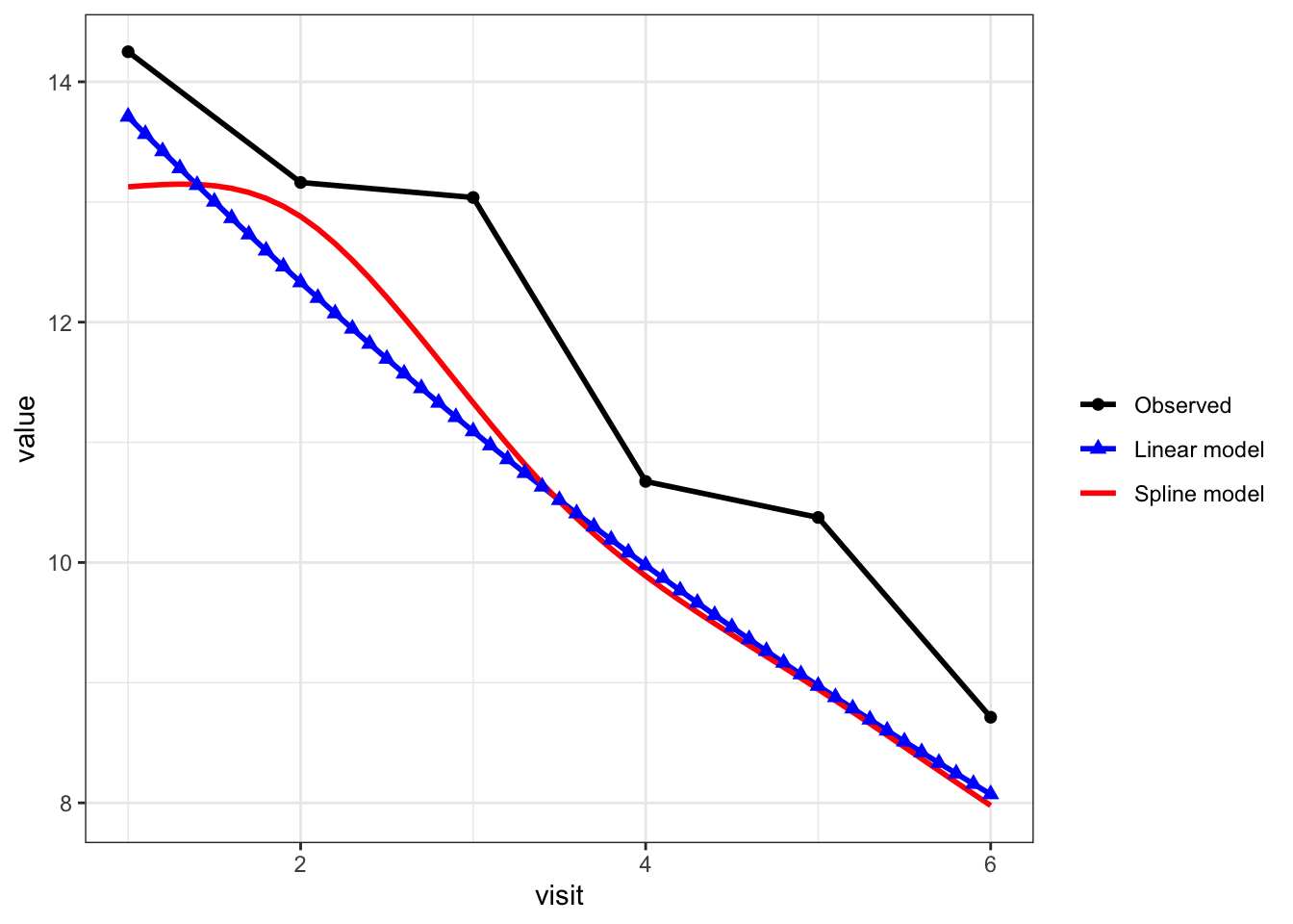
black line with circles = observed mean count at each visit
blue line with triangles = linear-time NB model
red line = spline-time NB model
The model-based predictions are slightly lower than the observed means because they represent the expected outcome for a typical subject (with average covariates and no subject-specific random effect), whereas the observed means average over heterogeneous subjects. As a result, differences between model-based predictions and raw means are expected and do not indicate poor model fit; the key comparison here is the trajectory over time rather than matching the raw means exactly.
Interpreting time effects across models:
# -----------------------------
# 16. Example contrasts between post-baseline visits
# -----------------------------

# For the spline model, compare predicted rates at selected visits.
# These are model-based comparisons across time points,
# conditional on baseline covariate being held fixed.

# Create dataset for selected visits
contrast_dat <- data.frame(
  visit = c(1, 2, 3, 4, 5, 6),   # <-- include all visits if you want all contrasts
  log_baseline = mean(dat$log_baseline),
  offset_log = 0,
  id = NA
)

# Get linear predictors (log scale)
lp <- predict(
  fit_spline,
  newdata = contrast_dat,
  type = "link",
  re.form = NA
)

# Compute rate ratios
rr_2_vs_1 <- exp(lp[2] - lp[1])
rr_3_vs_1 <- exp(lp[3] - lp[1])
rr_4_vs_1 <- exp(lp[4] - lp[1])
rr_5_vs_1 <- exp(lp[5] - lp[1])
rr_6_vs_1 <- exp(lp[6] - lp[1])

rr_4_vs_2 <- exp(lp[4] - lp[2])
rr_6_vs_4 <- exp(lp[6] - lp[4])

# cat("\nSpline model contrasts:\n")
# cat("Visit 2 vs Visit 1 rate ratio:", round(rr_2_vs_1, 3), "\n")
# cat("Visit 3 vs Visit 1 rate ratio:", round(rr_3_vs_1, 3), "\n")
# cat("Visit 4 vs Visit 1 rate ratio:", round(rr_4_vs_1, 3), "\n")
# cat("Visit 5 vs Visit 1 rate ratio:", round(rr_5_vs_1, 3), "\n")
# cat("Visit 6 vs Visit 1 rate ratio:", round(rr_6_vs_1, 3), "\n")
#
# cat("Visit 4 vs Visit 2 rate ratio:", round(rr_4_vs_2, 3), "\n")
# cat("Visit 6 vs Visit 4 rate ratio:", round(rr_6_vs_4, 3), "\n")

# These contrasts illustrate how the implied time effect can vary
# across different parts of follow-up when time is modeled flexibly.

# -----------------------------
# 17. Summarize true vs estimated effects
# -----------------------------

# --- 1. True effects (relative to visit 1) ---
true_rr <- exp(true_time_effect)

true_df <- data.frame(
  visit = as.numeric(names(true_rr)),
  true_rr_vs_v1 = as.numeric(true_rr)
)

# --- 2. Linear model estimate ---
beta_hat <- fixef(fit_linear)$cond["visit"]
rr_linear <- exp(beta_hat)

# Linear model implies cumulative effect per visit relative to visit 1
linear_df <- data.frame(
  visit = 1:6,
  linear_rr_vs_v1 = exp(beta_hat * (1:6 - 1))
)

# --- 3. Spline model estimates ---
contrast_dat <- data.frame(
  visit = 1:6,
  log_baseline = mean(dat$log_baseline),
  offset_log = 0,
  id = NA
)

lp <- predict(
  fit_spline,
  newdata = contrast_dat,
  type = "link",
  re.form = NA
)

spline_rr <- exp(lp - lp[1])

spline_df <- data.frame(
  visit = 1:6,
  spline_rr_vs_v1 = spline_rr
)

# --- Combine all ---
summary_table <- true_df %>%
  left_join(linear_df, by = "visit") %>%
  left_join(spline_df, by = "visit") %>%
  mutate(
    true_rr = round(true_rr_vs_v1, 3),
    linear_rr = round(linear_rr_vs_v1, 3),
    spline_rr = round(spline_rr_vs_v1, 3),

    true_pct = round(-(1 - true_rr) * 100, 1),
    linear_pct = round(-(1 - linear_rr) * 100, 1),
    spline_pct = round(-(1 - spline_rr) * 100, 1),

    `True RR (% reduction)` = paste0(true_rr, " (", true_pct, "%)"),
    `Linear model RR (% reduction)` = paste0(linear_rr, " (", linear_pct, "%)"),
    `Spline model RR (% reduction)` = paste0(spline_rr, " (", spline_pct, "%)")
  ) %>%
  select(
    `Visit` = visit,
    `True RR (% reduction)`,
    `Linear model RR (% reduction)`,
    `Spline model RR (% reduction)`
  )

knitr::kable(summary_table, align = "c")| Visit | True RR (% reduction) | Linear model RR (% reduction) | Spline model RR (% reduction) |
|---|---|---|---|
| 1 | 1 (0%) | 1 (0%) | 1 (0%) |
| 2 | 0.95 (-5%) | 0.899 (-10.1%) | 0.981 (-1.9%) |
| 3 | 0.9 (-10%) | 0.809 (-19.1%) | 0.863 (-13.7%) |
| 4 | 0.75 (-25%) | 0.728 (-27.2%) | 0.753 (-24.7%) |
| 5 | 0.75 (-25%) | 0.655 (-34.5%) | 0.682 (-31.8%) |
| 6 | 0.6 (-40%) | 0.589 (-41.1%) | 0.608 (-39.2%) |
The above table shows the rate ratio (% reduction) for each post-baseline visit relative to the first post-baseline visit. The linear time model assumes a constant rate ratio per visit (i.e., a constant multiplicative change between consecutive visits). However, when comparing each visit to the first post-baseline visit, these effects accumulate over time, resulting in different rate ratios at later visits (i.e., RR for visit 3 relative to visit 1 is \(0.8994^{2} \approx 0.728\)). Thus, while the per-visit effect is constant, the cumulative effect relative to visit 1 is not.
Because this is a single simulated dataset, the estimated effects are not expected to recover the true visit-specific effects exactly. The purpose here is to illustrate how different model specifications capture the longitudinal trajectory.
The two models capture the trajectory differently. The linear time model imposes a constant multiplicative change per visit, which accumulates over time and leads to increasingly large reductions at later visits. As a result, it overestimates % reduction when the true effect plateaus (e.g., visits 4–5).
In contrast, the spline model allows the trajectory to vary over time and better reflects the nonlinear pattern in the data, including smaller reductions at earlier visits and a subsequent plateau. While it does not recover the true visit-specific rate ratios exactly in this single simulated dataset, it provides a more flexible and realistic representation of the underlying trajectory.
This framework provides a more principled way to evaluate longitudinal seizure rate trajectory in single-arm studies:
What is a causal effect?
A causal effect is defined as the contrast between two potential outcomes for the same individual:
\[ Y(1) - Y(0) \]
where:
Because both potential outcomes cannot be observed for the same individual, causal effects cannot be directly measured. In a randomized trial, randomization allows unbiased estimation of the average causal effect by comparing outcomes between groups:
\[ E[Y(1) - Y(0)] \]
Apparent improvement measured as changes from baseline within a single arm may reflect natural fluctuations, regression to the mean, or other time effects, and does not identify a causal effect because it does not compare observed outcomes to the unobserved counterfactual.
uses all available data
respects the count nature of the outcome
incorporates baseline appropriately
allows flexible modelling of time
The model estimates how seizure rates evolve over time after treatment initiation.
However, it does not estimate a causal treatment effect defined as the contrast between two potential outcomes (see margin notes). In certain settings, such as rare diseases or areas of high unmet need, regulatory decisions may still rely on single-arm studies as supportive of efficacy when interpreted in the context of external evidence (e.g., natural history or historical controls). In these cases, the observed trajectory is used as part of a broader evidentiary framework rather than as a standalone estimate of causal effect.
In single-arm settings, changes from baseline (including PCFB and responder rates which are derived from PCFB) do not identify a treatment effect, as they conflate natural fluctuations, regression to the mean, or other time effects with treatment.
A longitudinal negative binomial model provides a more principled way to evaluate post-baseline trajectories by using all available data and accounting for baseline differences and within-subject variability. Importantly, how time is modelled matters. A linear time effect imposes a constant multiplicative change per visit, which can be overly restrictive and may misrepresent the underlying trajectory. Flexible approaches, such as splines, allow the data to inform how the post-baseline trajectory evolves over time. These models should be viewed as tools for describing longitudinal patterns, using time as a proxy for treatment exposure rather than establishing a causal treatment effect.
Hernán, M. A., & Robins, J. M. (2020). Causal inference: What if. Chapman & Hall/CRC.
Holland, P. W. (1986). Statistics and causal inference. Journal of the American Statistical Association, 81(396), 945–960. https://doi.org/10.1080/01621459.1986.10478354
Rubin, D. B. (1974). Estimating causal effects of treatments in randomized and nonrandomized studies. Journal of Educational Psychology, 66(5), 688–701. https://doi.org/10.1037/h0037350
U.S. Food and Drug Administration. (2023). Considerations for the design and conduct of externally controlled trials for drug and biological products (Draft Guidance). https://www.fda.gov/media/164960/download
U.S. Food and Drug Administration. (2019). Demonstrating substantial evidence of effectiveness for human drug and biological products (Draft Guidance). https://www.fda.gov/media/133660/download
U.S. Food and Drug Administration. (2019). Rare diseases: Natural history studies for drug development (Guidance for industry). https://www.fda.gov/media/122425/download